Producing a Trial Balance filtered for new accounts
Introduction
It is often useful to produce a Trial Balance report showing only those accounts which have been created in the period. This is a relatively straightforward exercise by taking an exported trial balance and filtering in excel. There are several steps, but in total the report should only take a couple of minutes to create once done once or twice. Unfortunately, this requires to be run on the second period of the year or after as it relies on the Year to Date being the same as the months transaction.
The steps are described below:-
Generate the Trial balance and export to Excel
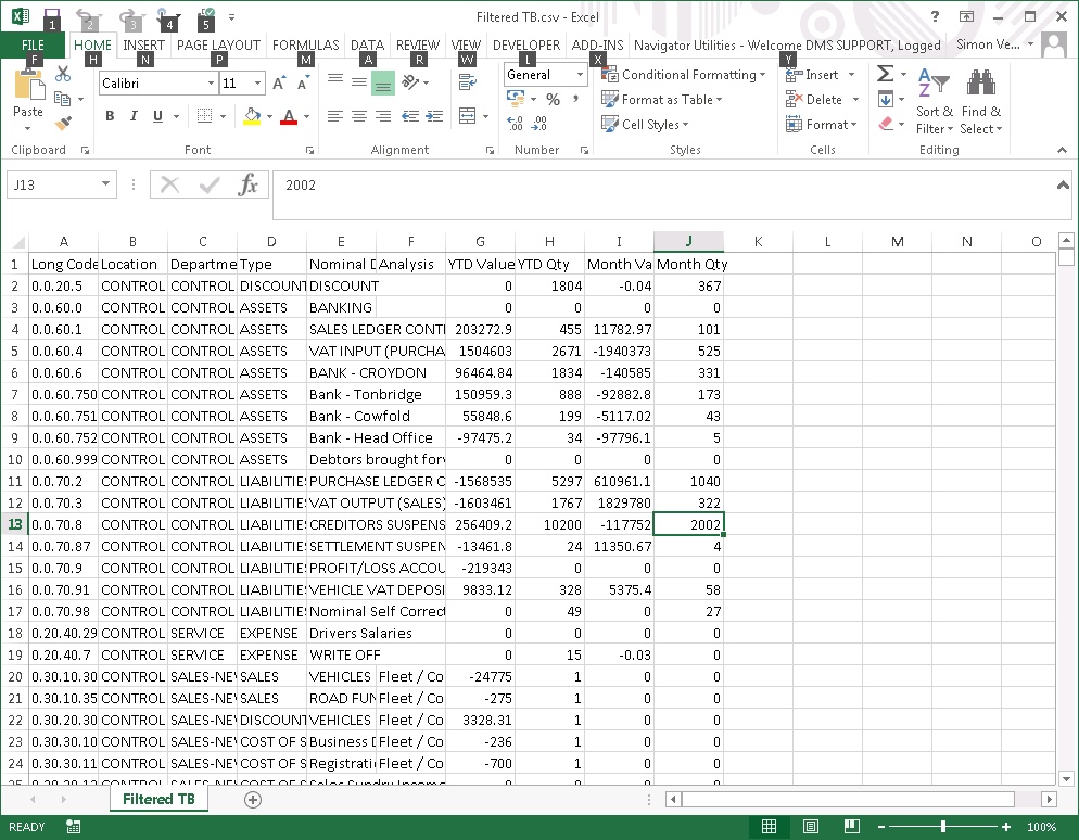
In Navigator, select Nominal Ledger > Reports > Ledger Reports. Select the Period no, and the “Extended Trial Balance” (this may be described slightly different on different systems). Then generate the report.
Once the report is on window, click the “Export” menu option at the top left of the window and click Export to Spreadsheet.
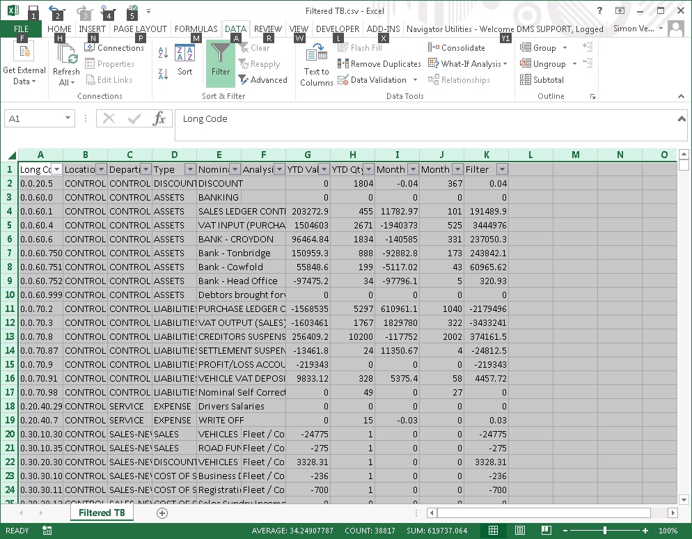
Navigator will request a filename. Enter a filename to save this report as. Once saved, Excel will automatically open up and display the Trial balance report :-
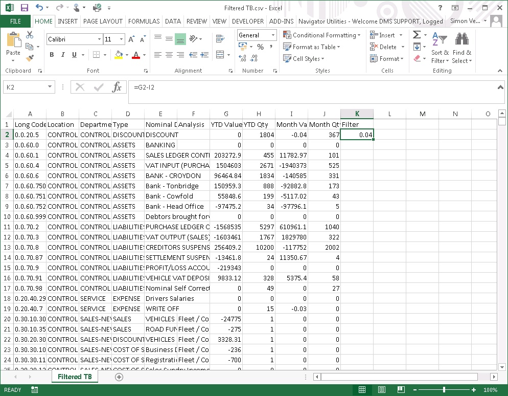
Add a column header at the end of the report called “Filter”
In this column, in row two enter a formula which subtracts the “month value” from the
“YTD value”. In the example above the formula would be : =G2-I2 (G refers to column G for YTD Value, and I refers to column I for Month Value). The spreadsheet will now look like :-
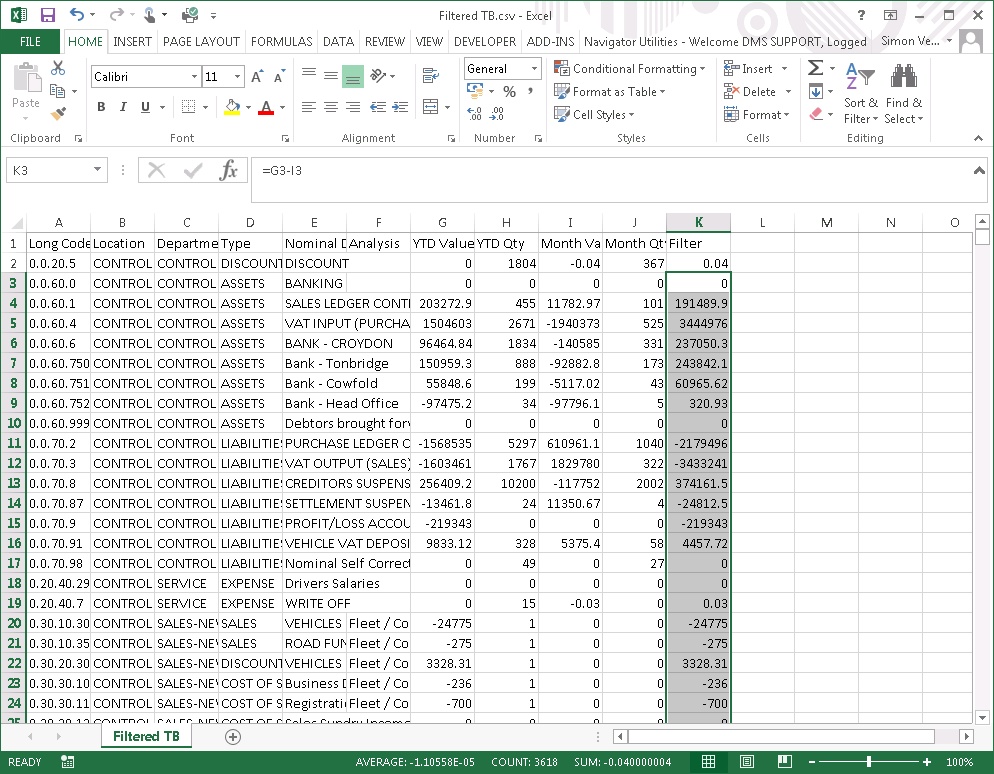
You now need to copy and paste the formula down all the whole of the filter column.
To do this, click in the box which has the formula in (K2 in this case) and press CTRL+C at the same time.
Then highlight the whole column by clicking in the box underneath, holding the shift key down whilst pressing “Page Down” to get to the end of the list, clicking in the last cell.
Press ENTER to copy the formula down. The spreadsheet will now look like :-
Now it is necessary to “Filter” the spreadsheet so that only columns with a YTD that is not zero and where the Filter column has a zero in are displayed.
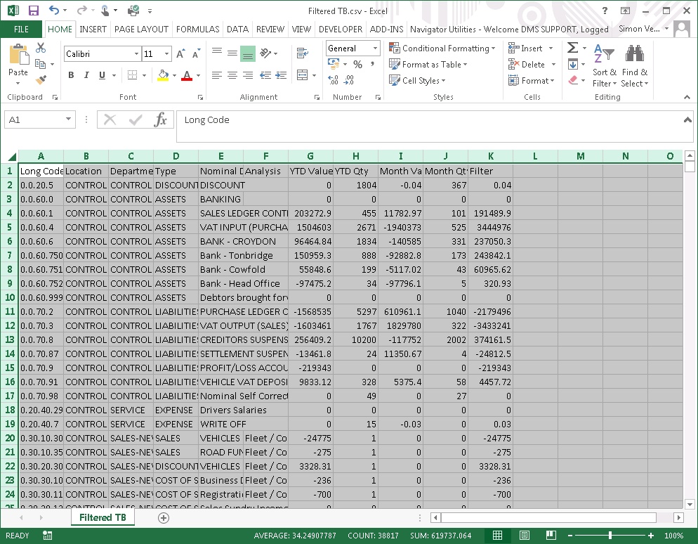
To do this, first click the left hand corner square (to the left of column heading A and above the row heading no 1). This will highlight all the cells in the spreadsheet :-
Now, click the Data Menu and the “Filter” option (described as “Autofilter” on older versions of Excel. This will produce a little “arrow” next to each column heading:
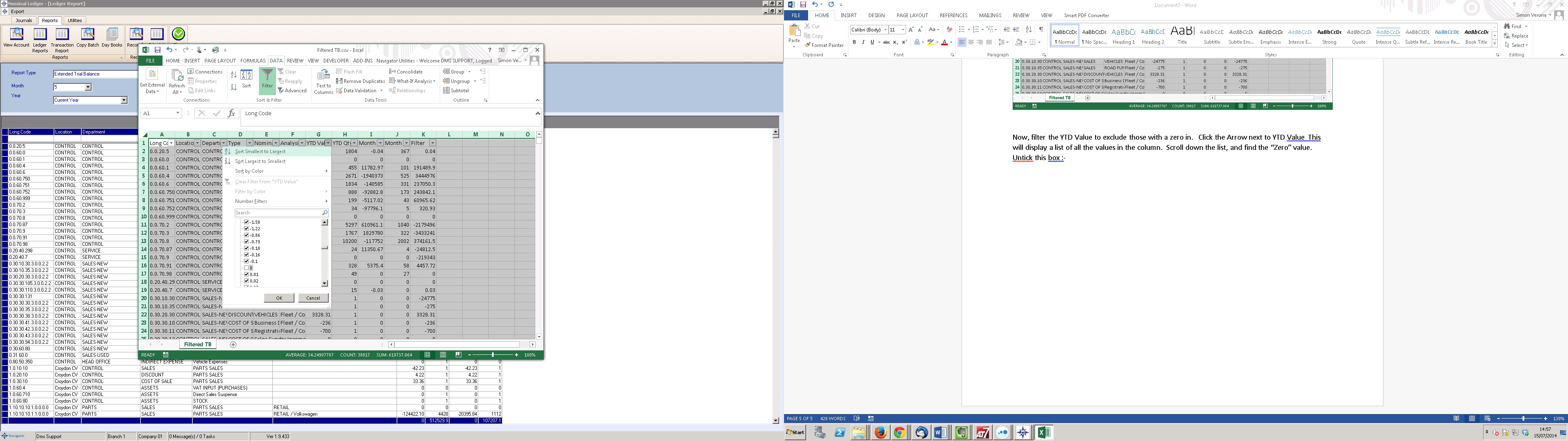
Now, filter the YTD Value to exclude those with a zero in. Click the Arrow next to YTD Value This will display a list of all the values in the column. Scroll down the list, and find the “Zero” value. Untick this box :-
Repeat the exercise for the filter column, but this time when filtering first untick the “Select All” tick box before then ticking the Zero box.
The spreadsheet will then look like :-
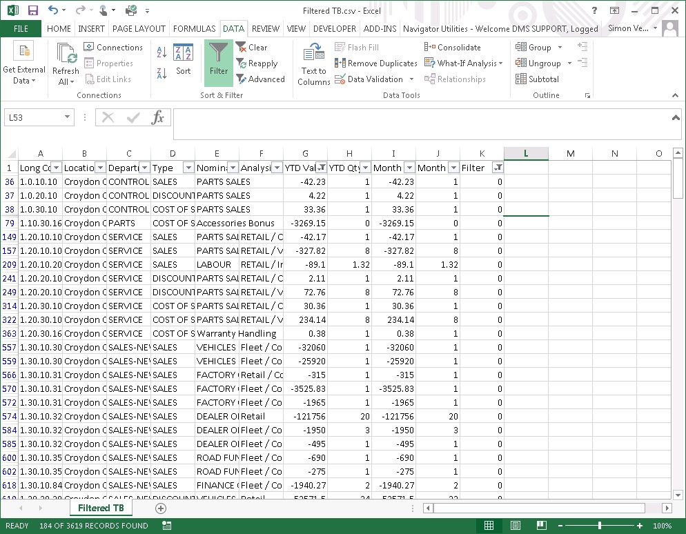
The filtering exercise is now complete. The only rows left showing are the new accounts used for the first time this month. Resize the columns to display as you need.